4. Predict observables and generate mocks#
Download this notebook (.ipynb) · Read the saved outputs here, or run the cells in Jupyter.
This notebook defines its own JAX model and physical parameters below. It builds on the model tutorial. Always distinguish a projected observable from an intrinsic quantity and a dispersion from a variance.
This notebook is self-contained. Install JeansPy with the numpyro_cpu and
plotting extras as described in the installation guide, then select that
environment as your Jupyter kernel and run cells from top to bottom.
Saved outputs are an example run; timings and short-chain results can vary.
Setup#
Run this setup in a fresh kernel. It defines all objects used below.
The generalized NFW halo uses ZhaoModel with fixed alpha=1, beta=3
and an untruncated cutoff. Its inner slope gamma is sampled in the
inference examples; truth["gamma"]=1 generates standard-NFW mocks.
import os
os.environ.setdefault("JEANSPY_JAX_PLATFORM", "cpu")
os.environ.setdefault("JEANSPY_JAX_ENABLE_X64", "true")

# The example uses no progress widgets; ignore only their optional-import warning.
import warnings
warnings.filterwarnings("ignore", message="IProgress not found.*")

# Import JeansPy before JAX so its runtime settings take effect.
from jeanspy.model_jax import (
    DSphModel, PlummerModel, ZhaoModel, ConstantAnisotropyModel,
)
from jeanspy.sampler_numpyro import JeansLikelihoodModel, ParameterSpec
import jax
import numpyro.distributions as dist
from numpyro.infer import MCMC, NUTS, init_to_value
import numpy as np
import matplotlib.pyplot as plt

model = DSphModel(submodels={
    "StellarModel": PlummerModel(),
    "DMModel": ZhaoModel(),
    "AnisotropyModel": ConstantAnisotropyModel(),
})
fixed = dict(re_pc=200., alpha=1., beta=3., r_t_pc=np.inf)
truth = dict(**fixed, rs_pc=500., rhos_Msunpc3=.1, gamma=1., beta_ani=0.)
options = dict(solver="kernel", n_u=128, n_kernel=32,
               dm_mass_method="numeric", dm_mass_n_steps=128)
rng = np.random.default_rng(123)
u = rng.uniform(size=32)
R_pc = 200. * np.sqrt(u / (1. - u))  # Projected Plummer radii.
e_vlos_kms = np.full(32, 2.)
variance = np.asarray(model.sigmalos2(R_pc, params=truth, **options))
vlos_kms = rng.normal(0., np.sqrt(variance + e_vlos_kms**2))
data = dict(R_pc=R_pc, vlos_kms=vlos_kms, e_vlos_kms=e_vlos_kms)
import jax.numpy as jnp
params = dict(truth)
Calculate the LOS dispersion#
import jax.numpy as jnp

variance = model.sigmalos2(R_pc, params=params, solver="kernel",
                          n_u=256, n_kernel=64)
sigma_kms = jnp.sqrt(variance)
sigmalos2 returns the intrinsic LOS second central moment in (km/s)².
The mean velocity does not belong inside its square root. NumPy users can
call model.sigmalos(R_pc, n=256, n_kernel=64) directly on a NumPy/SciPy model;
JAX users take the square root as above. The different keyword names are
documented in the individual
NumPy and
JAX API entries.
Plot a radial profile#
import numpy as np
import matplotlib.pyplot as plt

R_grid = np.geomspace(10., 3000., 100)
sigma_grid = np.sqrt(model.sigmalos2(
    R_grid, params=params, solver="kernel", n_u=256, n_kernel=64))
fig, ax = plt.subplots()
ax.semilogx(R_grid, sigma_grid)
ax.set(xlabel="Projected radius [pc]", ylabel=r"$\sigma_{los}$ [km/s]")
plt.show()
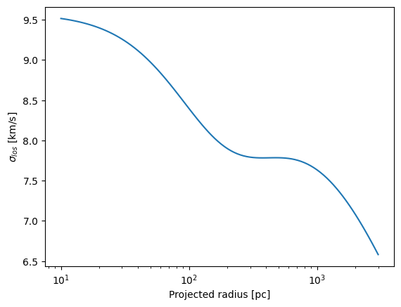
These host-side NumPy conversions are for plotting, after evaluation; keep
JAX operations inside a differentiated likelihood. To check numerical
stability, evaluate the same physical parameters and radii with larger
n_u and n_kernel and compare the predictions. A finer radius grid makes
the plot smoother but does not refine the underlying integration.
Inspect the components#
tracer = model["StellarModel"]
halo = model["DMModel"]
surface_density = tracer.density_2d(R_grid, re_pc=params["re_pc"])
r_grid = np.geomspace(10., 3000., 100)
spatial_density = tracer.density_3d(r_grid, re_pc=params["re_pc"])
halo_density = halo.mass_density_3d(r_grid, params=params)
mass = halo.enclosed_mass(r_grid, params=params)
The tracer densities are number-weighting functions; the halo density and mass set the potential. Halo density and mass methods can apply different cutoff conventions. Read the selected halo’s API entry before using its density in a custom integral. J/D factors additionally require a distance and an angular aperture; follow the factor guide.
Generate mock observations#
At a fixed observed radius, the Gaussian likelihood assumes
In this expression the second argument is the variance. NumPy’s
rng.normal expects its square root as scale. The Quickstart implements
this explicitly:
rng = np.random.default_rng(123)
u = rng.uniform(size=32)
R_pc = 200. * np.sqrt(u / (1. - u))  # Projected Plummer radii.
e_vlos_kms = np.full(32, 2.)
variance = np.asarray(model.sigmalos2(R_pc, params=truth, **options))
vlos_kms = rng.normal(0., np.sqrt(variance + e_vlos_kms**2))
data = dict(R_pc=R_pc, vlos_kms=vlos_kms, e_vlos_kms=e_vlos_kms)

R_grid = np.geomspace(10., 3000., 100)
sigma_kms = np.sqrt(model.sigmalos2(R_grid, params=truth, **options))
prediction, axes = plt.subplots(1, 2, figsize=(9, 3.5), layout="constrained")
axes[0].semilogx(R_grid, sigma_kms)
axes[0].set(xlabel="Projected radius [pc]", ylabel=r"$\sigma_{los}$ [km/s]")
axes[1].errorbar(R_pc, vlos_kms, yerr=e_vlos_kms, fmt=".")
axes[1].set(xscale="log", xlabel="Projected radius [pc]",
            ylabel="Observed LOS velocity [km/s]")
plt.show()
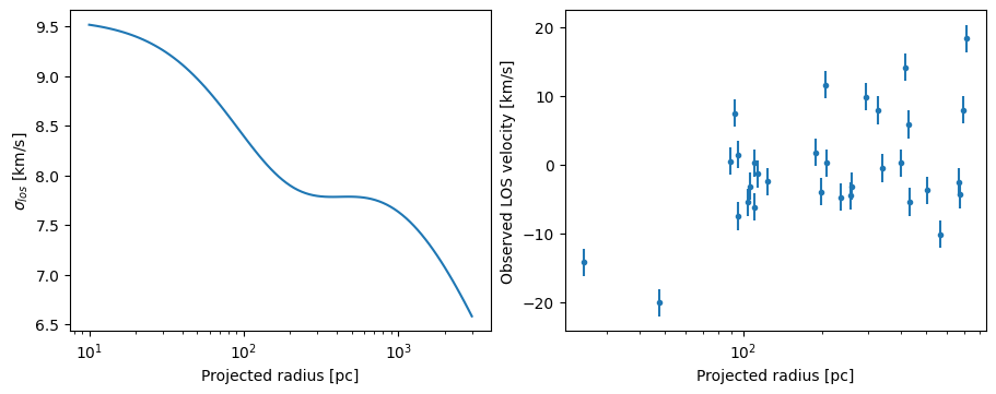
The setup above supplies fixed, truth and options for this mock.
The inverse Plummer CDF gives projected radii; real surveys may need spatial
selection, membership and measurement-error models. Generating Gaussian
velocities tests the assumed likelihood workflow, not a self-consistent
phase-space distribution. For an observed dataset the velocity likelihood
conditions on the supplied radii, so it does not also fit their distribution.