5. Run MCMC and inspect the posterior

Download this notebook (.ipynb) · Read the saved outputs here, or run the cells in Jupyter.

This notebook recreates the model and mock data from the Quickstart, so it can be run independently. The forward solver predicts a variance. Inference additionally requires a likelihood, sampling coordinates, priors and a sampling algorithm.

This notebook is self-contained. Install JeansPy with the numpyro_cpu and plotting extras as described in the installation guide, then select that environment as your Jupyter kernel and run cells from top to bottom. Saved outputs are an example run; timings and short-chain results can vary.

Setup

Run this setup in a fresh kernel. It defines all objects used below.

The generalized NFW halo uses ZhaoModel with fixed alpha=1, beta=3 and an untruncated cutoff. Its inner slope gamma is sampled in the inference examples; truth["gamma"]=1 generates standard-NFW mocks.

import os
os.environ.setdefault("JEANSPY_JAX_PLATFORM", "cpu")
os.environ.setdefault("JEANSPY_JAX_ENABLE_X64", "true")

# The example uses no progress widgets; ignore only their optional-import warning.
import warnings
warnings.filterwarnings("ignore", message="IProgress not found.*")

# Import JeansPy before JAX so its runtime settings take effect.
from jeanspy.model_jax import (
    DSphModel, PlummerModel, ZhaoModel, ConstantAnisotropyModel,
)
from jeanspy.sampler_numpyro import JeansLikelihoodModel, ParameterSpec
import jax
import numpyro.distributions as dist
from numpyro.infer import MCMC, NUTS, init_to_value
import numpy as np
import matplotlib.pyplot as plt

model = DSphModel(submodels={
    "StellarModel": PlummerModel(),
    "DMModel": ZhaoModel(),
    "AnisotropyModel": ConstantAnisotropyModel(),
})
fixed = dict(re_pc=200., alpha=1., beta=3., r_t_pc=np.inf)
truth = dict(**fixed, rs_pc=500., rhos_Msunpc3=.1, gamma=1., beta_ani=0.)
options = dict(solver="kernel", n_u=128, n_kernel=32,
               dm_mass_method="numeric", dm_mass_n_steps=128)

rng = np.random.default_rng(123)
u = rng.uniform(size=32)
R_pc = 200. * np.sqrt(u / (1. - u))  # Projected Plummer radii.
e_vlos_kms = np.full(32, 2.)
variance = np.asarray(model.sigmalos2(R_pc, params=truth, **options))
vlos_kms = rng.normal(0., np.sqrt(variance + e_vlos_kms**2))
data = dict(R_pc=R_pc, vlos_kms=vlos_kms, e_vlos_kms=e_vlos_kms)

Specify the likelihood

For independent Gaussian velocity errors, the likelihood used here is

\[ \log L(\theta)=-\frac12\sum_i\left[ \log(2\pi s_i^2)+\frac{(v_i-v_{\rm mem})^2}{s_i^2}\right], \qquad s_i^2=\sigma_{\rm los}^2(R_i;\theta)+\epsilon_i^2. \]

JeansLikelihoodModel implements this conditional velocity model for the JAX spherical solver. The tracer scale, alpha=1, beta=3 and the untruncated cutoff are fixed; the inner slope gamma is inferred. Thus the fit explores a generalized NFW family without marginalizing the tracer scale or outer slope. Membership, binaries and non-Gaussian velocity structure are not modeled here.

Choose sampling coordinates and priors

Sampled coordinate	Prior	Physical parameter supplied to the solver
log10_rs_pc	Uniform(1.5, 4)	rs_pc = 10**log10_rs_pc
log10_rhos_Msunpc3	Uniform(-3, 1)	rhos_Msunpc3 = 10**log10_rhos_Msunpc3
gamma	Uniform(0, 2)	Inner halo density slope
beta_ani	Uniform(-1, 0.75)	beta_ani
vmem_kms	Uniform(-50, 50)	Mean LOS velocity in km/s

Uniformity in a logarithm gives a log-uniform prior on the physical scale, not a uniform prior on that scale. ParameterSpec.pow10 samples the named logarithmic coordinate and transforms it for prediction. Do not add a Jacobian as though the distribution had instead been specified on the physical scale. Choose bounds for your scientific problem before fitting.

These independent priors span about 32–10,000 pc in rs_pc and 0.001–10 solar masses per pc³ in rhos_Msunpc3. The gamma prior includes cores and cusps; the mock uses gamma=1. With only 32 stars, radius, density, inner slope and anisotropy can remain degenerate. Inspect posterior sensitivity to the prior bounds rather than assuming the data constrain all five parameters. The broad anisotropy prior is a Jeans-moment example, not a guarantee of a nonnegative phase-space distribution.

dm_mass_method="numeric" keeps the Zhao enclosed mass differentiable with respect to gamma. Its resolution dm_mass_n_steps is separate from the LOS and anisotropy-kernel grids n_u and n_kernel. Refine all three on representative prior and posterior points before a scientific analysis; the NFW analytic mass path alone cannot fit an inner slope.

def physical_parameters(sampled):
    return {**fixed, **sampled}

likelihood = JeansLikelihoodModel(
    model,
    [ParameterSpec.pow10("log10_rs_pc", dist.Uniform(1.5, 4.), param_name="rs_pc"),
     ParameterSpec.pow10("log10_rhos_Msunpc3", dist.Uniform(-3., 1.),
                         param_name="rhos_Msunpc3"),
     ParameterSpec("gamma", dist.Uniform(0., 2.)),
     ParameterSpec("beta_ani", dist.Uniform(-1., .75)),
     ParameterSpec("vmem_kms", dist.Uniform(-50., 50.))],
    parameter_postprocess=physical_parameters,
    sigmalos2_kwargs=options,
)

parameter_postprocess assembles the spherical physical dictionary. Fixed and sampled names must not overlap. The axisymmetric likelihood instead also accepts fixed_params; read the selected constructor’s signature.

Run NumPyro NUTS

max_tree_depth = 10
kernel = NUTS(likelihood, target_accept_prob=.85, max_tree_depth=max_tree_depth,
              init_strategy=init_to_value(values={
                  "log10_rs_pc": np.log10(500.), "log10_rhos_Msunpc3": -1.,
                  "gamma": 1., "beta_ani": 0., "vmem_kms": 0.}))
mcmc = MCMC(kernel, num_warmup=200, num_samples=256,
            num_chains=2, chain_method="sequential", progress_bar=False)
mcmc.run(jax.random.PRNGKey(42), **data,
         extra_fields=("diverging", "energy", "num_steps", "accept_prob"))

num_warmup controls adaptation and num_samples is the number of saved post-warmup draws per chain. Sequential chains let this example run on one CPU device. The initial values are near the generating model because this is a mock example; real data require admissible initial values without knowing the answer. Use different initial regions when investigating mixing or multimodality.

Read the result without losing chain structure

names = ["log10_rs_pc", "log10_rhos_Msunpc3", "gamma", "beta_ani", "vmem_kms"]
mcmc.print_summary(exclude_deterministic=True)
posterior = mcmc.get_samples(group_by_chain=True)  # Each value: (chain, draw).
for name in names:
    interval = np.quantile(np.asarray(posterior[name]), [.16, .5, .84])
    print(name, "16%, 50%, 84%:", interval)
print("Divergences:", int(mcmc.get_extra_fields()["diverging"].sum()))

traces, axes = plt.subplots(len(names), 1, figsize=(7, 9), sharex=True, layout="constrained")
for i, name in enumerate(names):
    for chain_index, values in enumerate(np.asarray(posterior[name])):
        axes[i].plot(values, alpha=.8, lw=.7,
                     ls=["-", "--"][chain_index], label=f"Chain {chain_index + 1}")
    axes[i].set_ylabel(name)
axes[0].legend()
axes[-1].set_xlabel("Posterior draw (warmup excluded)")
plt.show()

                          mean       std    median      5.0%     95.0%     n_eff     r_hat
            beta_ani      0.26      0.42      0.38     -0.38      0.74    240.94      1.01
               gamma      0.83      0.47      0.81      0.00      1.46    168.39      1.01
  log10_rhos_Msunpc3     -1.57      0.83     -1.66     -2.99     -0.44    157.65      1.01
         log10_rs_pc      3.21      0.53      3.26      2.49      3.99    182.52      1.00
            vmem_kms     -0.35      1.55     -0.38     -2.81      2.24    432.42      1.00

Number of divergences: 0
log10_rs_pc 16%, 50%, 84%: [2.64120599 3.25927649 3.77525493]
log10_rhos_Msunpc3 16%, 50%, 84%: [-2.39459069 -1.65517657 -0.71662544]
gamma 16%, 50%, 84%: [0.29710162 0.80858003 1.31702316]
beta_ani 16%, 50%, 84%: [-0.21152182  0.37810021  0.65304241]
vmem_kms 16%, 50%, 84%: [-1.77938956 -0.37797063  1.17765941]
Divergences: 0

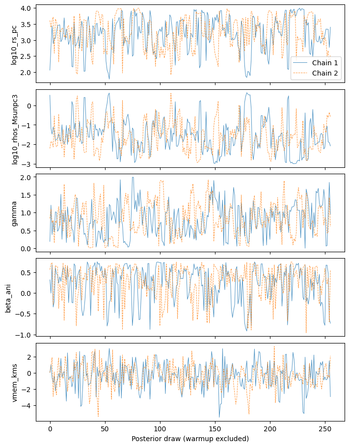
Check convergence and Monte Carlo precision

Keep (chain, draw) axes for diagnostics. Here ArviZ computes rank-normalized split R-hat, bulk ESS, tail ESS for the 5%/95% quantiles, and the Monte Carlo standard error (MCSE) of the mean. These are more informative than simply counting draws. The earlier NumPyro text summary uses its own diagnostic implementation; its rounded R-hat values need not equal this table.

Diagnostic	What to inspect	If it is poor
Trace / R-hat	Overlapping, stationary chains; R-hat near 1 (aim below 1.01)	Check separated modes and initial regions; improve parameterization/adaptation
Bulk / tail ESS	Sufficient effective draws for central / tail summaries	Increase draws after resolving sampling problems; examine slow correlations
MCSE	Simulation error small compared with the precision you need	Run longer when the sampler is otherwise reliable

For a final analysis, use at least four independently initialized chains; the two short chains here keep the walkthrough small. A useful initial ESS target is at least 100 effective draws per chain, then assess MCSE for the actual reported quantities. See the Stan diagnostic guidance and ArviZ R-hat definition.

import arviz as az
import pandas as pd

rows = []
for name in names:
    draws = np.asarray(posterior[name])  # Do not flatten chains here.
    rows.append(dict(parameter=name, r_hat=float(az.rhat(draws, method="rank")),
                     ess_bulk=float(az.ess(draws, method="bulk")),
                     ess_tail=float(az.ess(draws, method="tail", prob=(.05, .95))),
                     mcse_mean=float(az.mcse(draws, method="mean")),
                     posterior_sd=float(np.std(draws, ddof=1))))
diagnostics = pd.DataFrame(rows).set_index("parameter")
diagnostics["mcse_mean / sd"] = diagnostics.mcse_mean / diagnostics.posterior_sd
print(diagnostics.round(4).to_string())
print("Nonfinite diagnostics (investigate):",
      diagnostics.index[~np.isfinite(diagnostics).all(axis=1)].tolist())
print("R-hat >= 1.01:", diagnostics.index[diagnostics.r_hat >= 1.01].tolist())
print("Bulk ESS < 100 per chain:",
      diagnostics.index[diagnostics.ess_bulk < 100*mcmc.num_chains].tolist())
print("Tail ESS < 100 per chain:",
      diagnostics.index[diagnostics.ess_tail < 100*mcmc.num_chains].tolist())

                     r_hat  ess_bulk  ess_tail  mcse_mean  posterior_sd  mcse_mean / sd
parameter                                                                              
log10_rs_pc         1.0054  150.0313  109.4618     0.0393        0.5273          0.0744
log10_rhos_Msunpc3  1.0180  127.3284   88.8019     0.0660        0.8265          0.0799
gamma               1.0103  176.6550  221.2711     0.0361        0.4696          0.0768
beta_ani            1.0056  235.8798  194.5926     0.0271        0.4190          0.0648
vmem_kms            1.0030  459.4640  288.3247     0.0743        1.5465          0.0481
Nonfinite diagnostics (investigate): []
R-hat >= 1.01: ['log10_rhos_Msunpc3', 'gamma']
Bulk ESS < 100 per chain: ['log10_rs_pc', 'log10_rhos_Msunpc3', 'gamma']
Tail ESS < 100 per chain: ['log10_rs_pc', 'log10_rhos_Msunpc3', 'beta_ani']

Inspect NUTS divergences, energy and trajectory length

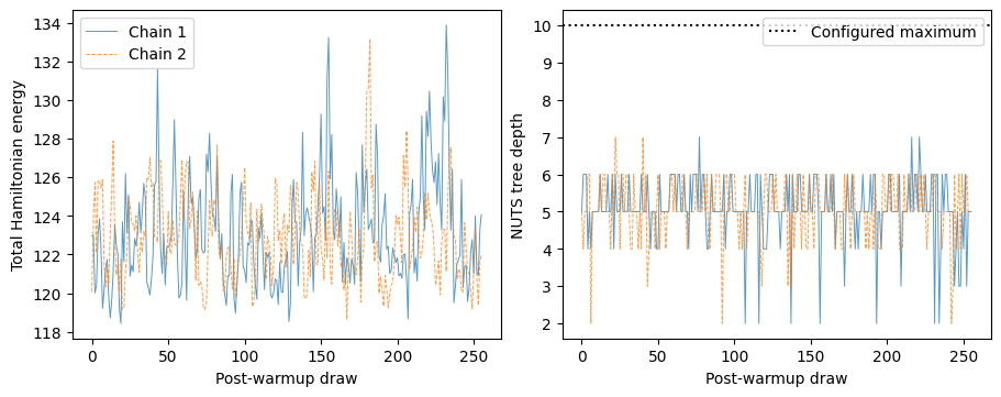
The extra_fields argument above records the diagnostics along with sampling; NumPyro otherwise does not save all of them. A divergence flags an inaccurate Hamiltonian trajectory and possible sampling bias. Check post-warmup counts per chain and their locations in parameter space, even when R-hat looks good.

BFMI uses total Hamiltonian energy, not just potential energy. Values below about 0.3 merit investigation. The tree-depth count below follows NumPyro’s documented relation to num_steps. Reaching the configured depth is an efficiency warning; it is distinct from a divergence. The mean acceptance probability is useful context but cannot certify convergence. See NumPyro’s MCMC fields and the ArviZ BFMI definition.

stats = {name: np.asarray(value) for name, value in
         mcmc.get_extra_fields(group_by_chain=True).items()}
diverging = stats["diverging"].astype(bool)
tree_depth = np.floor(np.log2(np.maximum(stats["num_steps"], 1))).astype(int) + 1
bfmi = np.asarray(az.bfmi(stats["energy"]))
nuts_diagnostics = pd.DataFrame({
    "divergences": diverging.sum(axis=1),
    "divergence_fraction": diverging.mean(axis=1),
    "BFMI": bfmi,
    "at_max_tree_depth": (tree_depth >= max_tree_depth).sum(axis=1),
    "mean_accept_prob": stats["accept_prob"].mean(axis=1),
}, index=pd.Index(np.arange(mcmc.num_chains)+1, name="chain"))
print(nuts_diagnostics.round(4).to_string())
print("All diagnostics exclude warmup.")

fig, axes = plt.subplots(1, 2, figsize=(9, 3.5), layout="constrained")
for chain in range(mcmc.num_chains):
    label = f"Chain {chain+1}"
    axes[0].plot(stats["energy"][chain], lw=.7, alpha=.75,
                 ls=["-", "--"][chain], label=label)
    axes[1].plot(tree_depth[chain], lw=.7, alpha=.75,
                 ls=["-", "--"][chain])
axes[0].set(ylabel="Total Hamiltonian energy", xlabel="Post-warmup draw")
axes[0].legend()
axes[1].axhline(max_tree_depth, color="black", ls=":", label="Configured maximum")
axes[1].set(ylabel="NUTS tree depth", xlabel="Post-warmup draw")
axes[1].legend()
plt.show()

       divergences  divergence_fraction    BFMI  at_max_tree_depth  mean_accept_prob
chain                                                                               
1                0                  0.0  0.8661                  0            0.9299
2                0                  0.0  0.8393                  0            0.9314
All diagnostics exclude warmup.

Locate correlations and divergences in a corner plot

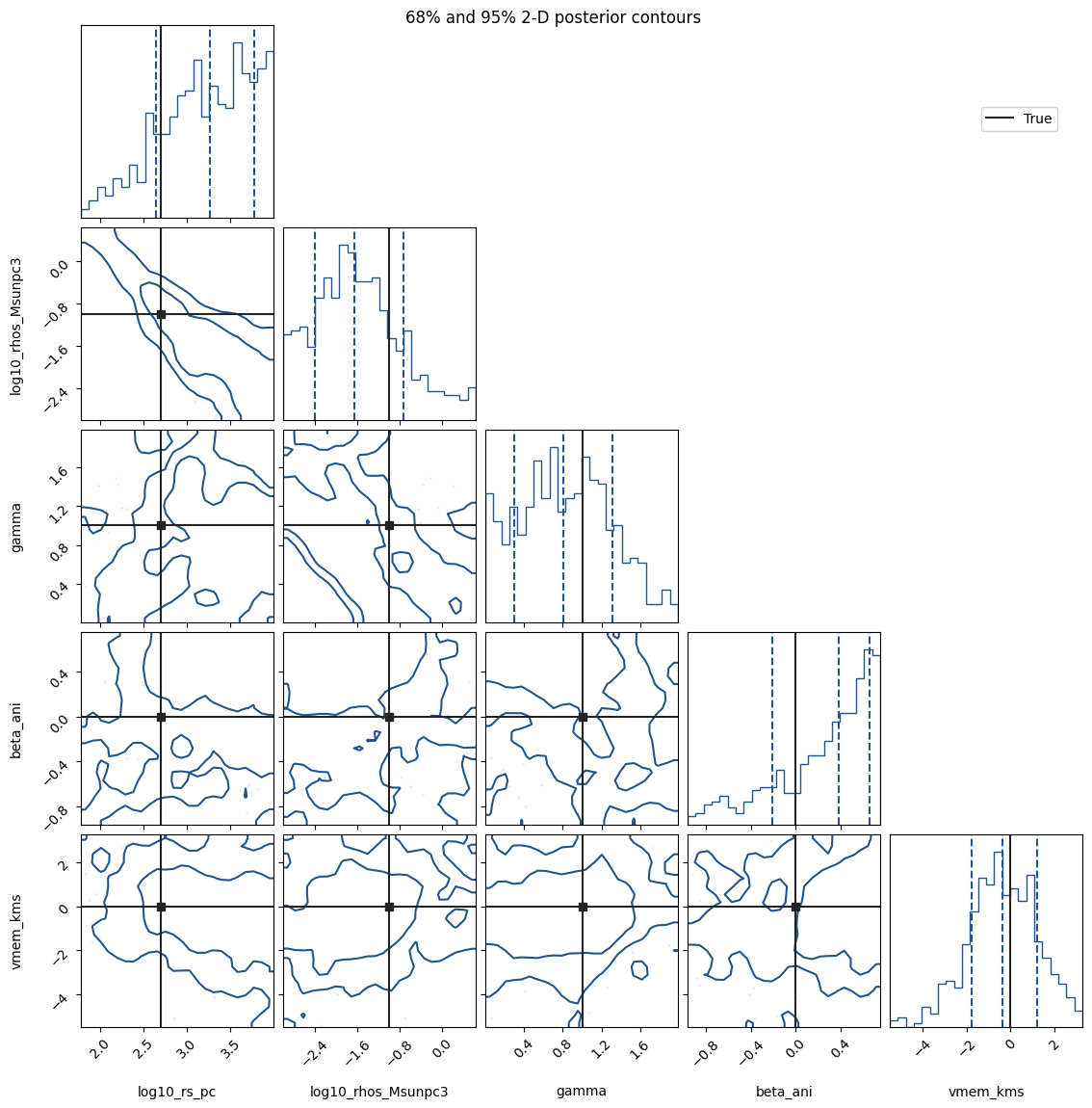
The lower triangle shows approximate 68% and 95% enclosed-probability contours of each 2-D marginal, estimated from smoothed histograms. They are not the default Gaussian-radius “1/2 sigma” levels and not a joint region in all five dimensions. Diagonal dashed lines show 16%, 50% and 84% marginal quantiles; black lines mark the true parameters. See the corner explanation of probability levels.

Flatten only for this plot, keeping the divergence mask in the same chain/draw order. Red crosses mark flagged post-warmup draws if any exist. If the count is zero, no red crosses are drawn; this is not a demonstration of a failed run. Do not discard divergent draws to make the plot look better. Their reported locations help diagnose geometry but do not trace the entire failed trajectory.

import corner
from matplotlib.lines import Line2D

flat = np.column_stack([np.asarray(posterior[name]).reshape(-1) for name in names])
divergent_flat = diverging.reshape(-1)
true_values = [np.log10(truth["rs_pc"]), np.log10(truth["rhos_Msunpc3"]),
               truth["gamma"], truth["beta_ani"], 0.]
fig = corner.corner(flat, labels=names, truths=true_values, truth_color="#242424",
                    levels=(.68, .95), bins=24, smooth=1.,
                    quantiles=(.16, .5, .84), color="#23558b",
                    plot_density=False, fill_contours=False,
                    label_kwargs={"fontsize": 10})
axes = np.asarray(fig.axes).reshape(len(names), len(names))
if divergent_flat.any():
    for i in range(len(names)):
        for j in range(i):
            axes[i, j].scatter(flat[divergent_flat, j], flat[divergent_flat, i],
                               marker="x", color="#b64635", s=20, zorder=5)
fig.suptitle("68% and 95% 2-D posterior contours", fontsize=12)
handles = [Line2D([], [], color="#242424", label="True")]
if divergent_flat.any():
    handles.append(Line2D([], [], marker="x", ls="none", color="#b64635", label="Divergent draw"))
fig.legend(handles=handles, loc="upper right", bbox_to_anchor=(.95, .9))
print("Flagged draws in the corner plot:", int(divergent_flat.sum()))
plt.show()

Flagged draws in the corner plot: 0

Decide what to change before trusting the posterior

Reading the recorded run: both chains have zero divergences and no depth-limit hits, and their BFMI values exceed 0.3. Nevertheless, log10_rhos_Msunpc3 and gamma have rank-normalized R-hat above 1.01, and several ESS values fall below the stated target. These short-run summaries and contours illustrate the workflow; they are not ready for final inference merely because the divergence count is zero.

If divergences occur, inspect their parameter-space pattern and verify finite, stable gradients and refined Jeans quadrature. A rerun with target_accept_prob=0.9 or 0.95 reduces step sizes, but difficult geometry may require reparameterization. For this radius/density degeneracy, adapting a dense mass matrix (dense_mass=True) is another option to investigate. See NumPyro’s posterior geometry tutorial. Record the change and compare diagnostics in a fresh run; changing a prior changes the inferential question and should have scientific justification.

For poor mixing without divergences, try more warmup, dispersed independent initializations and longer chains. Look for separate modes; blindly increasing max_tree_depth or dropping samples does not address the cause. Review low BFMI and frequent depth limits together with the geometry and energy traces.

Nonfinite diagnostics are unresolved, not a pass. Use the printed warnings from this short run as a worked example, not a pass/fail certificate. Inspect diagnostics for derived profiles too when they are the quantities to be reported. Good sampler diagnostics do not establish physical model adequacy or interval calibration; posterior predictive checks and, for calibration, repeated simulated datasets answer different questions.

The Quickstart profile plots propagate complete joint draws to dispersion and DM density. Their numerical MAP curve uses the posterior density in the named sampling coordinates; the pointwise posterior median generally is not the prediction at a single median parameter vector.

Use NumPy/SciPy with emcee

For the NumPy/SciPy backend, define the same physical model with stored parameters and a log posterior that updates them at each call. This example uses the same five sampling coordinates and Gaussian likelihood:

import emcee
from jeanspy.model import (
    DSphModel, PlummerModel, ZhaoModel, ConstantAnisotropyModel,
)
model = DSphModel(vmem_kms=0., submodels={
    "StellarModel": PlummerModel(re_pc=200.),
    "DMModel": ZhaoModel(rs_pc=500., rhos_Msunpc3=.1,
                         alpha=1., beta=3., gamma=1., r_t_pc=np.inf),
    "AnisotropyModel": ConstantAnisotropyModel(beta_ani=0.),
})
sigma_kms = np.sqrt(model.sigmalos2(R_pc, n=128, n_kernel=32))

# Sample halo radius, density, inner slope, anisotropy and systemic velocity.
# These illustrative priors are uniform in the named coordinates.
names = ["log10_rs_pc", "log10_rhos_Msunpc3", "gamma", "beta_ani", "vmem_kms"]
lower = np.array([1.5, -3., 0., -1., -50.])
upper = np.array([4., 1., 2., .75, 50.])


def log_probability(theta):
    if not np.all((lower < theta) & (theta < upper)):
        return -np.inf
    log_rs, log_rho, g, beta, mean = theta
    model.update(rs_pc=10**log_rs, rhos_Msunpc3=10**log_rho,
                 gamma=g, beta_ani=beta, vmem_kms=mean)
    variance = model.sigmalos2(R_pc, n=128, n_kernel=32) + e_vlos_kms**2
    return -.5 * np.sum(np.log(2*np.pi*variance) + (vlos_kms-mean)**2/variance)

Run the complete file from the checkout to include its imports, common mock data and output handling:

python examples/docs_quickstart_emcee.py --output-dir /tmp/jeanspy-emcee-example

Use a new output directory. The returned emcee chain has dimensions (step, walker, parameter); interacting walkers are not independent chains for R-hat. The JeansPy jeanspy.sampler.Sampler wrapper adds HDF5 storage and identity checks for supported estimation models. The direct emcee.EnsembleSampler route above lets you supply your own log posterior. For process pools, use a picklable callable and guard process creation with if __name__ == "__main__":; the local functions in the minimal Quickstart are not a multiprocessing example.

Next: save and resume results.

Check the emcee sampling interface

This short run exercises the emcee call on the same data. It does not establish convergence.

initial = np.array([np.log10(500.), -1., 1., 0., 0.])
walkers = initial + np.random.default_rng(42).normal(size=(16, len(names))) * [.05, .05, .05, .05, .5]
sampler = emcee.EnsembleSampler(16, len(names), log_probability)
sampler.random_state = np.random.RandomState(42).get_state()
sampler.run_mcmc(walkers, 32, progress=False)
print("(step, walker, parameter):", sampler.get_chain().shape)
assert np.all(np.isfinite(sampler.get_log_prob()))

(step, walker, parameter): (32, 16, 5)